Identifying Local Doping Patterns Around Atomic Sites

Introduction

Dopants and point defects play a pivotal role in tailoring material properties—from enhancing catalytic activity in metal oxides to shifting electronic bands in semiconductors. Traditional computational methods, such as full-lattice cluster expansions, supercell approaches, or large-scale Monte Carlo simulations, typically focus on global doping distributions across an entire crystal or supercell.

While these global techniques are essential for capturing macroscopic trends, the local coordination sphere often dominates the physics and chemistry of defects. For instance, in catalytic oxides, only atoms immediately adjacent to a dopant participate directly in reactions. In semiconductor physics, local defect complexes can introduce deep electronic levels that critically affect carrier lifetimes. Similarly, in solid electrolytes or ionic conductors, the clustering of dopants and vacancies typically occurs within the first or second coordination shells, significantly influencing ionic transport.

Moreover, dopants are frequently introduced at low concentrations in practical scenarios. Under these conditions, global symmetry in a large periodic supercell often breaks down locally, causing the dopant and its immediate coordination environment to exhibit reduced or entirely different symmetry compared to the parent crystal structure. Focusing specifically on a local cluster surrounding the dopant effectively circumvents the computational inconvenience associated with large periodic supercells, providing a more realistic representation of these site-specific distortions.

Additionally, from a computational standpoint, local doping patterns can be enumerated or sampled efficiently and rigorously. Such localized doping patterns can recur throughout the crystal structure, making this approach naturally scalable. Local configurations can be replicated or shifted to equivalent or near-equivalent sites without requiring extensive periodic supercells containing the dopant in every translational repeat, thereby avoiding a combinatorial explosion.

Code Description

Given the significance of local doping patterns, this blog presents a Python code designed to:

1. Identify Neighbors: Determine atomic species within a specified radius of a target site, forming the essential first step in analyzing the local atomic environment.

2. Utilize Symmetry: Leverage crystallographic site-symmetry operations to identify equivalent neighbor positions. This method eliminates redundancy by consolidating symmetrically equivalent doping configurations.

3. Generate Configurations with Controlled Composition: Perform exhaustive enumeration of all possible local doping arrangements in manageable systems. For more complex systems with extensive possibilities, employ quasi-random Sobol sampling to efficiently explore the configuration space while maintaining targeted dopant concentrations.

4. Represent and Visualize Patterns: Produce structured JSON outputs detailing unique doping patterns and neighbor orbits obtained through site-symmetry operations. Interactive visualization capabilities are provided via the crystaltoolkit package, allowing intuitive inspection of atomic arrangements.

Code Walkthrough

Below, I highlight the essential Python constructs that make the workflow possible.

Finding and Storing Neighbor Positions

After loading a structure (e.g., from a cif file) and selecting a target site site_index, the code lists all neighbors within a user-defined cutoff cutoff. It stores their fractional coordinates relative to the reference site:

structure = Structure.from_file("cubic_batio3.cif")
site_index = 0
cutoff = 7.0

target_site = structure[site_index]
neighbors = structure.get_sites_in_sphere(
    pt=target_site.coords,
    r=cutoff,
    include_index=True
)

rel_positions = []
neighbor_indices = []
for (site, dist, idx) in neighbors:
    if idx != site_index:
        rel_positions.append(
            structure.frac_coords[idx] - structure.frac_coords[site_index]
        )
        neighbor_indices.append(idx)
rel_positions = np.mod(rel_positions, 1.0)  # ensure within [0,1) for fractional coords

Building a KD-Tree and Mapping Symmetry Operations

To handle symmetry, the code retrieves the site-symmetry group:

sym_ops = get_site_symmetries(structure, site_index=site_index)

However, not all these operations are unique; some may differ by trivial translations. The code filters duplicates by comparing rotation matrices:

def get_unique_rotations(sym_ops, decimals: int = 6):
    unique_ops = []
    seen = set()
    for op in sym_ops:
        rot_flat = tuple(np.round(op.rotation_matrix.ravel(), decimals))
        if rot_flat not in seen:
            seen.add(rot_flat)
            unique_ops.append(op)
    return unique_ops

sym_ops = get_unique_rotations(sym_ops)

Next, the code sees how each operation permutes the neighbor list. It first builds a KD-tree from rel_positions:

def build_kdtree(rel_positions: np.ndarray) -> cKDTree:
    return cKDTree(rel_positions)

tree = build_kdtree(rel_positions)

Then, for each symmetry operation, the code transforms the relative positions and queries the KD-tree to identify which neighbor index best matches the transformed position:

def find_permutation(sym_op, rel_positions: np.ndarray, tree, rtol: float = 1e-2) -> List[int]:
    N = len(rel_positions)
    perm = [None] * N
    transformed = np.array([sym_op.operate(pos) for pos in rel_positions])
    transformed = np.mod(transformed, 1.0)  # keep fractional coords in [0,1)

    for i, tpos in enumerate(transformed):
        dist, idx = tree.query(tpos)
        if dist < rtol:
            perm[i] = idx
        else:
            # handle errors or no match cases
            pass
    return perm

By repeating this for every unique symmetry operation, the code collects a list of permutations mapping each neighbor index to another under the operation.

Orbits Under the Site-Symmetry Group

With permutations in hand, the code groups neighbor indices into orbits. Indices that map onto each other by any symmetry operation lie in the same orbit. This partitioning drastically reduces the number of distinct doping configurations:

def get_orbits_under_group(N: int, permutations: List[List[int]]) -> List[List[int]]:
    visited = [False] * N
    orbits = []

    for start_idx in range(N):
        if not visited[start_idx]:
            orbit = set()
            queue = [start_idx]
            while queue:
                current = queue.pop()
                if current not in orbit:
                    orbit.add(current)
                    visited[current] = True
                    for perm in permutations:
                        neighbor = perm[current]
                        if not visited[neighbor]:
                            queue.append(neighbor)
            orbits.append(sorted(orbit))
    return orbits

Enumerating or Sampling Doping Patterns

Suppose I have a doping_dict that specifies which elements can be replaced and by what dopants. For instance:

doping_dict = {
  "Ba": ["Ba", "Sr"],
  "Ti": ["Ti", "Zr"]
}

If a neighbor is originally "Ba", it can become "Ba" or "Sr"; if it is "Ti", it can become "Ti" or "Zr". After grouping neighbors into orbits, I can enumerate doping assignments within each orbit and apply backtracking to avoid counting symmetry-equivalent patterns multiple times.

For large orbits or numerous dopant species, enumeration can become huge. The code checks if the total number of combinations exceeds a threshold (e.g., 1e6). If it does, it uses quasi-random Sobol sampling to ensure coverage while respecting doping fraction constraints.

Applying Doping Fraction Constraints

Constraints of the form

"doping_fraction_constraints": {
  "Sr": [0.0, 0.3],
  "Zr": [0.0, 0.5]
}

ensure, for example, that the overall fraction of "Sr" among the dopable neighbor sites lies between 0.0 and 0.3. The code checks each final labeling to ensure it meets these fraction bounds before accepting it into the final set.

Example Usage

Below are two common ways to use this code: command-line or direct Python import.

Command-Line

1. Structure Input: Provide a cif file or other supported format for your crystal.
   

2. Configuration JSON: Specify doping species and fraction constraints

3. Run:

   python find_doping_pattern.py \
     --structure cubic_batio3.cif \
     --site-index 0 \
     --cutoff 7.0 \
     --config-json doping_config.json \
     --max-enum-threshold 1000000 \
     --output results.json

The script identifies neighbors of site 0 up to 7 Å, enumerates doping patterns (or samples them if above the threshold 1e6), and saves unique configurations to results.json.

Python Usage

You can also import a driver function in your own Python workflow:

from doping_analysis import run_doping_analysis
from pymatgen.core import Structure

structure = Structure.from_file("cubic_batio3.cif")

doping_dict = {"Ba": ["Ba", "Sr"], "Ti": ["Ti", "Zr"]}
doping_fraction_constraints = {"Sr": (0.0, 0.3), "Zr": (0.0, 0.5)}

results = run_doping_analysis(
    structure=structure,
    site_index=0,
    cutoff=7.0,
    doping_dict=doping_dict,
    doping_fraction_constraints=doping_fraction_constraints,
    max_enum_threshold=1_000_000
)

print("Number of final patterns:", len(results["final_patterns"]))
print("Orbits:", results["orbits"])

Interactive Visualization

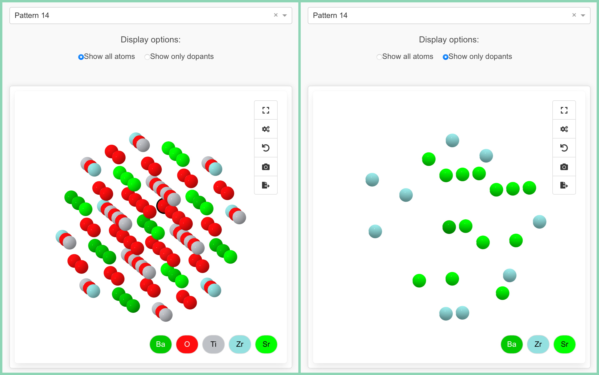
To help users explore and understand the generated doping patterns, the code includes an interactive visualization interface built with Dash and Crystal Toolkit. The visualization component allows you to:

1. Select Different Patterns: Browse through all generated doping patterns using a dropdown menu
2. Display Options: Toggle between showing all atoms or only the dopant atoms
3. 3D Interaction: Rotate, zoom, and pan to examine the local atomic environment from any angle

Example Doping Pattern Visualization (left) all atoms, (right) only dopants

How This Code Could Be Used

1. DFT Cluster Setup
   By enumerating unique local doping patterns, you can generate input structures for small-cluster or supercell-based ab initio calculations, ensuring that you capture all relevant local doping motifs (without duplicates) near a site of interest.

2. Machine Learning Training Data
   When training ML potentials or neural network force fields, coverage of doped environments is essential. This code systematically creates local doping configurations to feed into high-fidelity calculations (e.g., DFT) for label generation.

3. High-Throughput Screening
   Researchers exploring doping across multiple materials or sites can automate the pipeline: for each material, each site, and each doping fraction range, the script enumerates or samples doping arrangements.

4. Local Defect Complex Analysis
   In ion conductors or oxide-based electrolytes (like ceria or zirconia), dopants often cluster with oxygen vacancies. With minor modifications (e.g., including "Vac" as a valid species), you can systematically explore dopant–vacancy complexes.

5. Interfacing with Cluster Expansion
   Even if you eventually plan a global cluster expansion, having a library of local dopant environments is valuable for building an initial pool of training structures that sufficiently represent local doping motifs.